Portfolio Optimization with Python: Modern Portfolio Theory

For a machine-learning based portfolio optimization algorithm, see this post.

In a previous post, we covered portfolio optimization and its implementations in R. In this post, We will tackle the problem of portfolio optimization using Python, which offers some elegant implementations. Much of the structure of the post is gleaned from Yves Hilpisch’s awesome book Python for Finance. Our analysis essentially boils down to the following tasks:

Import financial data via API’s
Compute returns and statistics
Simulate a random set of portfolios
Construct a set of optimal portfolios using Markowitz’s mean-variance framework
Visualize the set of optimal portfolios using the plotly library
Backtest the performance of the optimal portfolio

Tools from The Python Ecosystems

We need the following Python libraries and packages:

Show code

[project]
name = "portfolio-opt"
version = "0.1.0"
requires-python = ">=3.11"
dependencies = [
    "matplotlib>=3.9.2",
    "pandas[performance]>=2.2.3",
    "plotly>=6.2.0",
    "pyfolio>=0.9.2",
    "scipy>=1.14.1",
    "yfinance>=0.2.46",
]

[tool.uv]
package = false

[dependency-groups]
notebook = [
    "ipykernel>=6.29.5",
]
lint-fmt = [
    "ruff>=0.7.0",
]

Show code

from datetime import datetime, timedelta
import numpy as np
import pandas as pd
import yfinance as yf
import scipy.optimize as sco
import scipy.interpolate as sci
import matplotlib.pyplot as plt
import matplotlib.ticker as ticker
import plotly.graph_objects as go
import plotly.offline as pyo
pyo.init_notebook_mode(connected=True)

{'text/html': '        <script type="text/javascript">\n        window.PlotlyConfig = {MathJaxConfig: \'local\'};\n        if (window.MathJax && window.MathJax.Hub && window.MathJax.Hub.Config) {window.MathJax.Hub.Config({SVG: {font: "STIX-Web"}});}\n        </script>\n        <script type="module">import "https://cdn.plot.ly/plotly-3.0.1.min"</script>\n        '}

Daily Prices and Returns

For our sample, we select 12 different equity assets with exposure to all of the GICS sectors— energy, materials, industrials, utilities, healthcare, financials, consumer discretionary, consumer staples, information technology, communication services, and real estate. The sampling period will cover the last 10 years, starting from 2021-09-15, ensuring comprehensive historical data for analysis.

Show code

# Create a list of symbols
symbols = [
  "XOM", "SHW", "JPM", "AEP", "UNH", "AMZN", 
  "KO", "BA", "AMT", "DD", "TSN", "SLG"
]
end_date = datetime(2021, 9, 15)
start_date = (end_date - timedelta(days = 365 * 10)).strftime('%Y-%m-%d')

daily_prices = yf.download(
  tickers = ' '.join(symbols), 
  start = start_date,
  end = end_date.strftime('%Y-%m-%d'),
  auto_adjust=False
)["Adj Close"]


[                       0%                       ]
[********              17%                       ]  2 of 12 completed
[************          25%                       ]  3 of 12 completed
[****************      33%                       ]  4 of 12 completed
[********************  42%                       ]  5 of 12 completed
[**********************50%                       ]  6 of 12 completed
[**********************58%***                    ]  7 of 12 completed
[**********************67%*******                ]  8 of 12 completed
[**********************75%***********            ]  9 of 12 completed
[**********************83%***************        ]  10 of 12 completed
[**********************92%*******************    ]  11 of 12 completed
[*********************100%***********************]  12 of 12 completed

Show code

daily_prices.columns = symbols

dates	XOM	SHW	JPM	AEP	UNH	AMZN	KO	BA	AMT	DD	TSN	SLG
2011-09-18	22.27761	41.12045	12.0845	52.15866	27.24173	22.11518	23.03708	21.70486	38.53153	13.19113	40.34365	42.96294
2011-09-19	22.74061	41.07578	11.6625	51.67896	26.79950	21.95181	23.08937	21.57695	38.34211	12.87742	40.24673	43.14365
2011-09-20	22.23013	40.29373	11.5935	49.61374	25.09935	20.65172	22.64163	20.76306	35.72952	12.56371	38.77676	41.95445
2011-09-21	22.01050	38.95310	11.1615	47.74367	22.62283	19.92340	22.16448	20.34449	33.39545	12.47954	38.03370	40.36302
2011-09-22	22.23013	38.94563	11.1805	48.38600	23.12404	20.14121	22.03376	20.74853	33.70185	12.57901	38.44560	40.40381

Next, we find the simple daily returns for each of the 12 assets using the pct_change() method, since our data object is a Pandas DataFrame. We use simple returns since they have the property of being asset-additive, which is necessary since we need to compute portfolios returns:

Show code

# Compute daily simple returns
daily_returns = (
  daily_prices.pct_change()
            .dropna(
              # Drop the first row since we have NaN's
              axis = 0,
              how = 'any',
              inplace = False
            )
)

dates	XOM	SHW	JPM	AEP	UNH	AMZN	KO	BA	AMT	DD	TSN	SLG
2011-09-19	0.0207836	-0.0010863	-0.0349208	-0.0091970	-0.0162336	-0.0073872	0.0022698	-0.0058929	-0.0049160	-0.0237821	-0.0024025	0.0042062
2011-09-20	-0.0224483	-0.0190391	-0.0059164	-0.0399623	-0.0634398	-0.0592247	-0.0193914	-0.0377205	-0.0681388	-0.0243610	-0.0365238	-0.0275638
2011-09-21	-0.0098798	-0.0332715	-0.0372623	-0.0376927	-0.0986685	-0.0352669	-0.0210739	-0.0201592	-0.0653261	-0.0066994	-0.0191627	-0.0379323
2011-09-22	0.0099784	-0.0001917	0.0017023	0.0134537	0.0221549	0.0109327	-0.0058978	0.0198599	0.0091749	0.0079709	0.0108300	0.0010107
2011-09-25	0.0085445	0.0231403	0.0279058	0.0420096	0.0416490	0.0696181	0.0198755	0.0686469	0.0231405	0.0273722	0.0254204	0.0347717

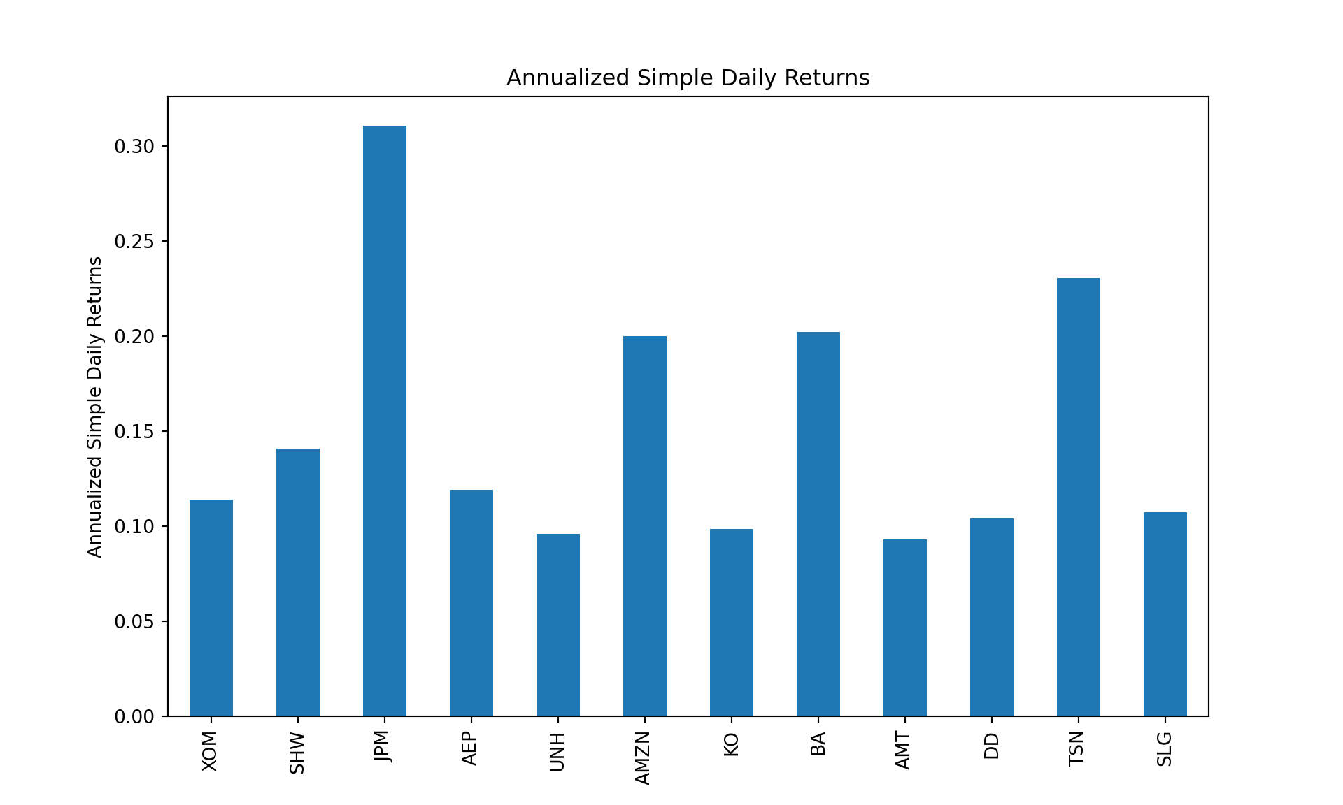
The simple daily returns may be visualized using line charts, density plots, and histograms, which are covered in my other post on visualizing asset data. Even though the visualizations in that post use the ggplot2 package in R, the plotnine package, or any other Python graphics librarires, can be employed to produce them in Python. For now, let us annualize the daily returns over the 10-year period ending in 2025-08-10. We assume the number of trading days in a year is computed as follows:

$365.25 (days on average per year) \times 57 (proportion work days per week) - 6 (weekday holidays) - 3 \times 57 (fixed date holidays) = 252.75 \approx 253$

Show code

annualized_simple_daily_returns = daily_returns.mean() * 253

fig, ax = plt.subplots(figsize=(10, 6))

# Plot the annualized simple daily returns
annualized_simple_daily_returns.plot(kind='bar', ax=ax);
ax.set_title('Annualized Simple Daily Returns');
ax.set_ylabel('Annualized Simple Daily Returns');
plt.show()

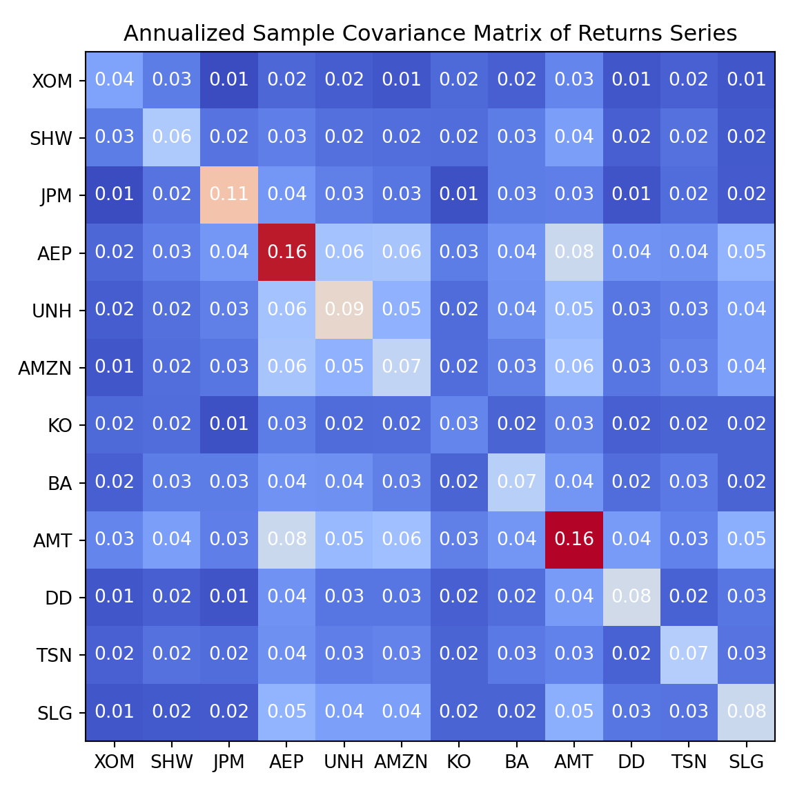
As can be seen, there are significant differences in the annualized performances between these assets. The annualized variance-covariance matrix of the returns can be computed using built-in pandas method cov. Note that while the sample covariance matrix is an unbiased estimator of the population covariance matrix, it can be subject to significant estimation error, especially when the number of assets is large relative to the number of observations. In our case, because of the relatively long sample period, the estimation error is likely to be small:

Show code

annualized_sample_covariance = daily_returns.cov() * 253

fig, ax = plt.subplots();
cax = ax.matshow(annualized_sample_covariance, cmap="coolwarm");
ax.xaxis.set_ticks_position('bottom');
ax.set_xticks(np.arange(len(annualized_sample_covariance.columns)));
ax.set_yticks(np.arange(len(annualized_sample_covariance.columns)));
ax.set_xticklabels(annualized_sample_covariance.columns);
ax.set_yticklabels(annualized_sample_covariance.columns);

for i in range(annualized_sample_covariance.shape[0]):
    for j in range(annualized_sample_covariance.shape[1]):
        # Ensure text can be easily seen
        value = annualized_sample_covariance.iloc[i, j]
        color = "white" if value < 0.5 else "black"
        ax.text(j, i, f"{value:.2f}", ha="center", va="center", color=color);

plt.title("Annualized Sample Covariance Matrix of Returns Series");
plt.tight_layout();
plt.show()

The variance-covariance matrix of the returns will be needed to compute the variance of the portfolio returns.

The Optimization Problem

The portfolio optimization problem, therefore, given a universe of assets and their characteristics, deals with a method to spread the capital between them in a way that maximizes the return of the portfolio per unit of risk taken. There is no unique solution for this problem, but a set of solutions, which together define what is called an efficient frontier— the portfolios whose returns cannot be improved without increasing risk, or the portfolios where risk cannot be reduced without reducing returns as well. The Markowitz model for the solution of the portfolio optimization problem has a twin objective of maximizing return and minimizing risk, built on the Mean-Variance framework of asset returns and holding the basic constraints, which reduces to the following:

Minimize Risk given Levels of Return

$min \to w \sqrt \to w T ˆ Σ \to w$

subject to

$\to w T ˆ μ = ˉ r P \to w T \to 1 = 1 (Full investment) \to 0 \leq \to w \leq \to 1 (Long only)$

Maximize Return given Levels of Risk

$max \to w \to w T ˆ μ$

subject to

$\to w T ˆ Σ \to w = ˉ σ P \to w T \to 1 = 1 (Full investment) \to 0 \leq \to w \leq \to 1 (Long only)$

In absence of other constraints, the above model is loosely referred to as the “unconstrained” portfolio optimization model. Solving the mathematical model yields a set of optimal weights representing a set of optimal portfolios. The solution set to these two problems is a hyperbola that depicts the efficient frontier in the $μ - σ$ -diagram.

Monte Carlo Simulation

The first task is to simulate a random set of portfolios to visualize the risk-return profiles of our given set of assets. To carry out the Monte Carlo simulation, we define two functions that both take as inputs a vector of asset weights and output the annualized expected portfolio return and standard deviation:

Annualized Returns

Show code

# Function for computing portfolio return
def portfolio_returns(weights) -> float:
    return float((np.sum(daily_returns.mean() * weights)) * 253)

Annualized Standard Deviation

Show code

# Function for computing standard deviation of portfolio returns
def portfolio_sd(weights) -> float:
    return float(np.sqrt(np.transpose(weights) @ (daily_returns.cov() * 253) @ weights))

Next, we use a for loop to simulate random vectors of asset weights, computing the expected portfolio return and standard deviation for each permutation of random weights. Again, we ensure that each random weight vector is subject to the long-positions-only and full-investment constraints.

Monte Carlo Simulation

The empty containers we instantiate are lists, which are mutable. This makes python lists more memory efficient than growing vectors in R, provided the number of simulations isn’t excessively large (i.e., in the millions). In such cases, resizing and over-allocation costs would be huge, and we should vectorize the potoflio_returns and portfolio_sd functions to leverage NumPy’s vectorized operations.

Show code

num_portfolios = 5000
num_assets = len(symbols)

# Generate random weights for all portfolios
random_weights = np.random.random((num_portfolios, num_assets))
# Normalize the weights so that the sum of weights for each portfolio equals 1
random_weights /= np.sum(random_weights, axis=1, keepdims=True)

list_portfolio_returns = []
list_portfolio_sd = []

# Monte Carlo simulation: loop through each set of random weights
for weights in random_weights:
    list_portfolio_returns.append(portfolio_returns(weights))  # Calculate and store returns
    list_portfolio_sd.append(portfolio_sd(weights))  # Calculate and store standard deviations (risk)

port_returns = np.array(list_portfolio_returns)
port_sd = np.array(list_portfolio_sd)

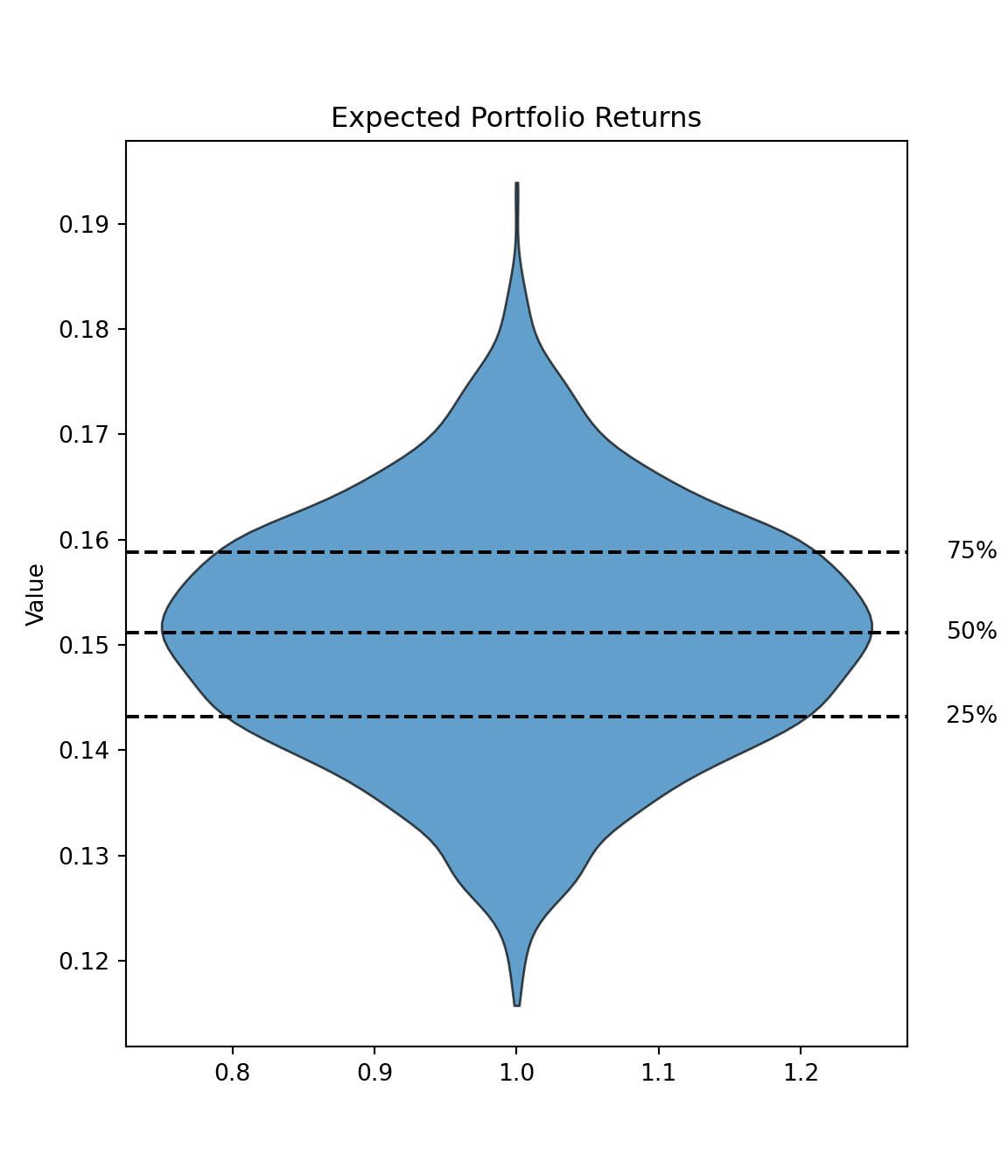
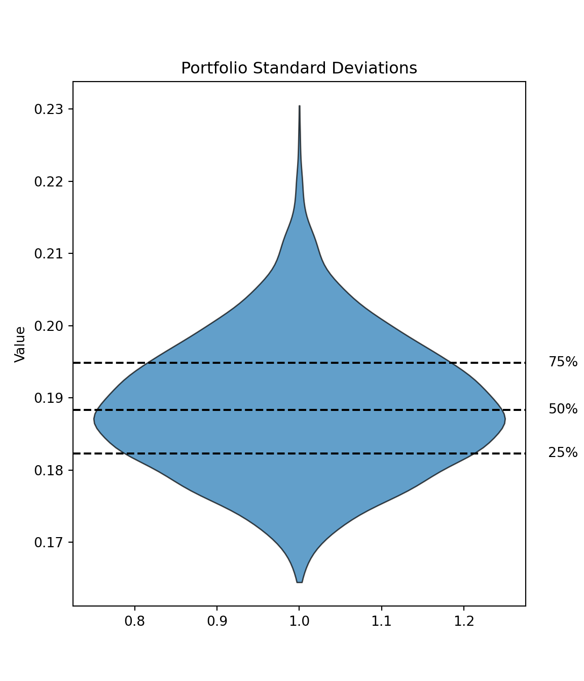
Let us examine the simulation results. In particular, the highest and the lowest expected portfolio returns are as follows:

Show code

def plot_violin_with_quantiles(data: np.ndarray, title: str) -> None:
    fig, ax = plt.subplots(figsize=(6, 7))
    parts = ax.violinplot(data, showmeans=False, showmedians=False, showextrema=False)

    # Customize the violin plot appearance
    for pc in parts['bodies']:
        pc.set_facecolor('#1f77b4')
        pc.set_edgecolor('black')
        pc.set_alpha(0.7)

    # Calculate and annotate quantiles
    quantiles = np.percentile(data, [25, 50, 75])
    for q, label in zip(quantiles, ['25%', '50%', '75%']):
        ax.axhline(q, color='black', linestyle='--')
        ax.text(1.05, q, f'{label}', transform=ax.get_yaxis_transform(), ha='left', va='center')

    # Set labels and title
    ax.set_ylabel('Value')
    ax.set_title(title)
    plt.show()

Show code

plot_violin_with_quantiles(port_returns, 'Expected Portfolio Returns')

Show code

plot_violin_with_quantiles(port_sd, 'Portfolio Standard Deviations')

We may also visualize the expected returns and standard deviations on a $μ - σ$ trade-off diagram:

Show code

sharpe = port_returns / port_sd

fig = go.Figure(
    data=go.Scattergl(
        x=port_sd,
        y=port_returns,
        mode='markers',
        marker=dict(
            size=5,
            opacity=0.7,
            color=sharpe,
            colorscale='Viridis',
            colorbar=dict(title='Sharpe Ratio')
        )
    )
);

fig.update_layout(
    title='Mean–Standard Deviation Diagram',
    paper_bgcolor='rgba(0,0,0,0)',  
    plot_bgcolor='rgba(0,0,0,0)', 
    xaxis=dict(
        title='Portfolio Standard Deviation (Annualized)',
        tickformat='.2%',
        showgrid=True,
        gridcolor='lightgray',
        gridwidth=1,
    ),
    yaxis=dict(
        title='Expected Portfolio Return (Annualized)',
        tickformat='.2%',
        showgrid=True,
        gridcolor='lightgray',
        gridwidth=1,
    ),
    showlegend=False
);

fig.show()

Each point in the diagram above represents a permutation of expected-return-standard-deviation value pair. The points are color coded such that the magnitudes of the Sharpe ratios, defined as $S R \equiv μ P - r f σ P$ , can be readily observed for each expected-return-standard-deviation pairing. For simplicity, we assume that $r f \equiv 0$ . It could be argued that the assumption here is restrictive, so I explored using a different risk-free rate in my previous post.

The Optimal Portfolios

Solving the optimization problem defined earlier provides us with a set of optimal portfolios given the characteristics of our assets. There are two important portfolios that we may be interested in constructing— the minimum variance portfolio and the maximal Sharpe ratio portfolio. In the case of the maximal Sharpe ratio portfolio, the objective function we wish to maximize is our user-defined Sharpe ratio function. The constraint is that all weights sum up to 1. We also specify that the weights are bound between 0 and 1. In order to use the minimization function from the SciPy library, we need to transform the maximization problem into one of minimization. In other words, the negative value of the Sharpe ratio is minimized to find the maximum value; the optimal portfolio composition is therefore the array of weights that yields that maximum value of the Sharpe ratio.

Show code

# User defined Sharpe ratio function
# Negative sign to compute the negative value of Sharpe ratio
def sharpe_fun(weights):
  return - (portfolio_returns(weights) / portfolio_sd(weights))

We will use a list of dictionaries to represent the constraints:

Show code

# We use an anonymous lambda function
constraints = [{'type': 'eq', 'fun': lambda x: np.sum(x) - 1}]

Next, the bound values for the weights:

Show code

# This creates 12 tuples of (0, 1), creating a sequence of (min, max) pairs
bounds = tuple(
  (0, 1) for w in weights
)

We also need to supply a starting sequences of weights, which essentially functions as an initial guesses. For our purposes, this will be an equal weight array:

Show code

# Repeat the list with the value (1 / 12) 12 times, and convert list to array
equal_weights = np.array(
  [1 / len(symbols)] * len(symbols)
)

We will use the scipy.optimize.minimize function and the Sequential Least Squares Programming (SLSQP) method for the minimization:

Show code

# Minimization results
max_sharpe_results = sco.minimize(
  # Objective function
  fun = sharpe_fun, 
  # Initial guess, which is the equal weight array
  x0 = equal_weights, 
  method = 'SLSQP',
  bounds = bounds, 
  constraints = constraints
)

The optimization results is an isntance of scipy.optimize.optimize.OptimizeResult, which contains many objects. The object of interest to us is the weight composition array, which we employ to construct the maximal Sharpe ratio portfolio:

Show code

# Extract the weight composition array
max_sharpe_results["x"]

array([9.18924204e-02, 1.13898648e-01, 2.16503565e-01, 0.00000000e+00,
       2.96034439e-16, 0.00000000e+00, 0.00000000e+00, 3.04707960e-01,
       0.00000000e+00, 9.55735829e-02, 1.77423824e-01, 4.90325473e-17])

Check that the weights sum to 1:

Show code

np.allclose(np.sum(max_sharpe_results["x"]), 1, atol=1e-12)

True

Maximal Sharpe Ratio Portfolio

The expected return, standard deviation, and Sharpe ratio of the maximal Sharpe ratio portfolio are as follows:

Show code

max_sharpe_port_return = portfolio_returns(max_sharpe_results["x"])
max_sharpe_port_sd = portfolio_sd(max_sharpe_results["x"])
pd.DataFrame(
  {
    "Expected Return": [max_sharpe_port_return],
    "Standard Deviation": [max_sharpe_port_sd],
    "Sharpe Ratio": [max_sharpe_port_return / max_sharpe_port_sd]
  }
)

   Expected Return  Standard Deviation  Sharpe Ratio
0          0.26003            0.174889      1.486826

Minimum Variance Portfolio

The minimum variance portfolio may be constructed similarly. The objective function, in this case, is the standard deviation function:

Show code

# Minimize sd
min_sd_results = sco.minimize(
  # Objective function
  fun = portfolio_sd, 
  # Initial guess, which is the equal weight array
  x0 = equal_weights, 
  method = 'SLSQP',
  bounds = bounds, 
  constraints = constraints
)

The expected return, standard deviation, and Sharpe ratio of the minimum variance portfolio are as follows:

Show code

min_sd_port_return = portfolio_returns(min_sd_results["x"])
min_sd_port_sd = portfolio_sd(min_sd_results["x"])
pd.DataFrame(
  {
    "Expected Return": [min_sd_port_return],
    "Standard Deviation": [min_sd_port_sd],
    "Sharpe Ratio": [min_sd_port_return / min_sd_port_sd]
  }
)

   Expected Return  Standard Deviation  Sharpe Ratio
0         0.162526            0.148197      1.096689

Efficient Frontier

As an investor, one is generally interested in the maximum return given a fixed risk level or the minimum risk given a fixed return expectation. As mentioned in the earlier section, the set of optimal portfolios— whose expected portfolio returns for a defined level of risk cannot be surpassed by any other portfolio— depicts the so-called efficient frontier. The Python implementation is to fix a target return level and, for each such level, minimize the volatility value. For the optimization, we essentially “fit” the twin-objective described earlier into an optimization problem that can be solved using quadratic programming. (The objective function is the portfolio standard deviation formula, which is a quadratic function) Therefore, the two linear constraints are the target return (a linear function) and that the weights must sum to 1 (another linear function). We will again use a tuple of dictionaries to represent the constraints:

Show code

# The arguments x will be the weights
constraints = (
  {'type': 'eq', 'fun': lambda x: portfolio_returns(x) - target}, 
  {'type': 'eq', 'fun': lambda x: np.sum(x) - 1}
)

The full-investment and long-positions-only specifications will remain unchanged throughout the optimization process, but the value the name target is bound to will be different during each iteration. Since dictionaries are mutable, the first constraint dictionary will be updated repeatedly during the minimization process. However, because tuples are immutable, the references held by the constraints tuple will always point to the same objects. This nuance makes the implementation Pythonic. We constrain the weights such that all weights fall within the interval $[0, 1]$ :

Show code

bounds = tuple(
  (0, 1) for w in weights
)

We will use the scipy.optimize.minimize function again and the Sequential Least Squares Programming (SLSQP) method for the minimization:

Show code

# Initialize an array of target returns
target = np.linspace(
  start = 0.15, 
  stop = 0.30,
  num = 100
)

obj_sd = []
for target in target:
  # Minimize the twin-objective function given the target expected return
  min_result_object = sco.minimize(
    fun = portfolio_sd, 
    x0 = equal_weights, 
    method = 'SLSQP',
    bounds = bounds, 
    constraints = constraints
    )
  # Extract the objective value and append it to the output container
  obj_sd.append(min_result_object['fun'])

obj_sd = np.array(obj_sd)
# Rebind target to a new array object
target = np.linspace(
  start = 0.15, 
  stop = 0.30,
  num = 100
)

When we plot the efficient frontier, we may wish to highlight the two portfolios in the plot— the maximal Sharpe ratio and the minimum variance portfolios:

Show code

sharpe = port_returns / port_sd
ef_sharpe = target / obj_sd
max_sharpe = max_sharpe_port_return / max_sharpe_port_sd
min_sharpe = min_sd_port_return / min_sd_port_sd

fig = go.Figure()

# All portfolios
fig.add_trace(
    go.Scattergl(
        x=port_sd,
        y=port_returns,
        mode="markers",
        marker=dict(
            size=5,
            opacity=0.7,
            color=sharpe,
            colorscale="Viridis",
            colorbar=dict(title="Sharpe Ratio"),
        ),
        showlegend=False,
    )
);

# efficient frontier
fig.add_trace(
    go.Scattergl(
        x=obj_sd,
        y=target,
        mode="markers",
        marker=dict(size=7, color=ef_sharpe, colorscale="Viridis", showscale=False),
        showlegend=False,
    )
);

# Maximal‐Sharpe portfolio
fig.add_trace(
    go.Scattergl(
        x=[max_sharpe_port_sd],
        y=[max_sharpe_port_return],
        mode="markers",
        marker=dict(size=7, color=[max_sharpe], colorscale="Viridis", showscale=False),
        showlegend=False,
    )
);

# Minimum‐variance portfolio
fig.add_trace(
    go.Scattergl(
        x=[min_sd_port_sd],
        y=[min_sd_port_return],
        mode="markers",
        marker=dict(size=7, color=[min_sharpe], colorscale="Viridis", showscale=False),
        showlegend=False,
    )
);

fig.update_layout(
    title="Mean–Standard Deviation Diagram",
    paper_bgcolor='rgba(0,0,0,0)',  
    plot_bgcolor='rgba(0,0,0,0)', 
    xaxis=dict(
      title="Portfolio Standard Deviation (Annualized)", 
      tickformat=".2%", 
      showgrid=True, 
      gridcolor='lightgray', 
      gridwidth=1,
    ),
    yaxis=dict(
      title="Expected Portfolio Return (Annualized)", 
      tickformat=".2%", 
      showgrid=True, 
      gridcolor='lightgray', 
      gridwidth=1,
    ),
);

fig.update_layout(
    annotations=[
        dict(
            x=max_sharpe_port_sd,
            y=max_sharpe_port_return,
            text="Maximal Sharpe Ratio Portfolio",
            xref="x",
            yref="y",
            showarrow=True,
            arrowhead=5,
            arrowsize=0.5,
            ax=20,
            ay=-40,
        ),
        dict(
            x=min_sd_port_sd,
            y=min_sd_port_return,
            text="Minimum Variance Portfolio",
            xref="x",
            yref="y",
            showarrow=True,
            arrowhead=5,
            arrowsize=0.5,
            ax=20,
            ay=-40,
        ),
    ]
);

fig.show()

Evidently, the efficient frontier is comprised of all optimal portfolios with a higher return than the global minimum variance portfolio. These portfolios dominate all other sub-optimal portfolios in terms of expected returns given a certain risk level.

Capital Market Line

Now that we have determined a set of efficient portfolios of risky assets, we may be interested in adding a risk-free asset to the mix. By adjusting the wealth allocation for the risk-free asset, it is possible for us to achieve any risk-return profile that lies on the straight line (in the $μ - σ$ diagram) between the risk-free asset and an efficient portfolio. This is called the capital market line, which is drawn from the point of the risk-free asset to the feasible region for risky assets. The capital market line has the equation:

$R p = r f + R T - r f σ T σ p$

where

$R p = portfolio return$
$r f = risk free rate$
$R T = market return$
$σ T = standard deviation of market portfolio$
$σ p = standard deviation of portfolio$

The problem then becomes: which efficient portfolio on the efficient frontier should we use? The answer is the tangency portfolio, at which point on the efficient frontier the slope of the tangent line is equal to that of the capital market line. In order to find the slope of the tangent line, a functional approximation of the efficient frontier and its first derivative must be obtained. Yves Hilpisch’s book recommends the use of cubic splines interpolation to obtain a continuously differentiable functional approximation of the efficient frontier, $f (x)$ . To carry out cubic splines interpolation, we need to create two array objects representing the expected returns and standard deviations of each of the efficient portfolios on the efficient frontier. In other words, we need to exclude from obj_sd and target (our two arrays of optimization results) the portfolios whose standard deviations are greater than that of the minimum variance portfolio but whose expected returns are smaller; they are not optimal and are therefore not on the efficient frontier:

Show code

# Use np.argmin() to find the index of the minimum variance portfolio and take a slice starting from that point, excluding previous elements
efficient_sd = obj_sd[np.argmin(a = obj_sd):]

# Take a slice of target returns starting from the minimum variance portfolio index and exclude previous elements
efficient_returns = target[np.argmin(a = obj_sd):]

We will leverage the the facilities from the scipy.interpolate sub-package, in particular, the splrep() function. Given the set of data points $(x i, y i)$ , the scipy.interpolate.splrep() function determine a smooth spline approximation of degree $k$ . The function will return a tuple $(t, c, k)$ with three elements— the vector of knots $t$ , the B-spline coefficients $c$ , and the degree of the spline $k$ .

Show code

# Cubic spline interpolation
tck = sci.splrep(
  x = np.sort(efficient_sd),
  y = efficient_returns,
  k = 3
)

Next, we use the scipy.interpolate.splev() function to define the functional approximation and the first derivative of the efficient frontier— $f (x)$ and $f' (x)$ . Given the knots and the B-spline coefficients, the function scipy.interpolate.splev() evaluates the value of the smoothing polynomial and its derivative:

Show code

# Define functional approximation of efficient frontier
def f(x):
  return sci.splev(
  x = x,
  tck = tck,
  der = 0
  )
# Define first derivative of the efficient frontier
def df(x):
  return sci.splev(
  x = x,
  tck = tck,
  der = 1
  )

Let us re-examine the equation for the capital market line. Notice that the line is a linear equation of the form:

$f (x) = a + b x$

where the parameters are as follows:

$a = r f$
$b = R T - r f σ T = f' (x) Slope of the capital market line = slope of the tangent line of the efficient frontier$
$x = σ p$

There are three unknown parameters and therefore we must have three equations to solve for the values of these parameters:

$a = r f ⟹ 0 = r f - a b = f' (x) ⟹ 0 = b - f' (x) f (x) = a + b x ⟹ 0 = a + b \cdot x - f (x)$

To solve the system, we will use the scipy.optimize.fsolve() function, which finds the roots of any input function. First, we need to define a function that returns the values of all three equations given a set of parameters $p = (a, b, x)$ . The set of parameters $p$ can be represented using a python list where $p [0] = a$ , $p [1] = b$ , and $p [2] = x$ :

Show code

# System of equations
def sys_eq(p, r_f = 0.01):
  # Equations
  eq1 = r_f - p[0]
  eq2 = p[1] - df(p[2])
  eq3 = r_f + df(p[2]) * p[2] -  f(p[2])
  # Output values
  return eq1, eq2, eq3

The function scipy.optimize.fsolve() returns an ndarray object, which is the solution set to the linear system above:

Show code

# Solve the linear system
sol_set = sco.fsolve(
  # Equations to solve for
  func = sys_eq,
  # Initial guess for p
  # This can be determined by trial and error or from the plot above (may take more than one try)
  x0 = [0.05, 1, 0.15]
)

As a sanity check, we an plug our solution set into our user defined function sys_eq to see if the results are indeed zeros:

Show code

# Sanity check
np.round(
  sys_eq(
    p = sol_set
  ),
  4
)

array([ 0., -0.,  0.])

We have confirmed that our solution set for the linear system is as follows:

$a =$ 0.01
$b =$ 1.4299
$x =$ 0.1766

Tangency Portfolio

To find the tangency portfolio, we use the same routine when we solved for the efficient frontier. We can compute the target return using the $x$ value from our solution set above. The rest is exactly the same as before.

The fun key of the first contstraint dictionary now uses the f (functional approximation of the efficient frontier) function and $x$ (the value of the solution set) to compute the target return:

Show code

# Constraints
constraints = (
  {'type': 'eq', 'fun': lambda x: portfolio_returns(x) - f(x = sol_set[2])}, 
  {'type': 'eq', 'fun': lambda x: np.sum(x) - 1}
)

min_result_object_tangency = sco.minimize(
  fun = portfolio_sd, 
  x0 = equal_weights, 
  method = 'SLSQP',
  bounds = bounds, 
  constraints = constraints
)

The expected return, standard deviation, and Sharpe ratio of the tangency portfolio are as follows:

Show code

tangency_port_return = portfolio_returns(min_result_object_tangency["x"])
tangency_port_sd = portfolio_sd(min_result_object_tangency["x"])
pd.DataFrame(
  {
    "Expected Return": [tangency_port_return],
    "Standard Deviation": [tangency_port_sd],
    "Sharpe Ratio": [tangency_port_return / tangency_port_sd]
  }
)

   Expected Return  Standard Deviation  Sharpe Ratio
0         0.262572            0.176635      1.486528

Finally, with these parameters, we can now plot the capital market line on the $μ - σ$ diagram. Similar to our approach earlier, we first define a function $g (x)$ whose body is the linear equation of the capital market line. This function takes as its argument the x values of the $μ - σ$ diagram:

Show code

# Capital market line
def cml(x):
  return sol_set[0] + sol_set[1] * x

Next, create arrays of plotting data:

Show code

# Standard deviations
cml_sd = np.linspace(
  start = 0, 
  stop = 0.25,
  num = 100
)
# Expected returns
cml_exp_returns = cml(x = cml_sd)

Move to R and plot the capital market line on the $μ - σ$ diagram:

Show code

sharpe = port_returns / port_sd
ef_sharpe = target / obj_sd

fig = go.Figure()

# All random portfolios
fig.add_trace(
    go.Scattergl(
        x=port_sd,
        y=port_returns,
        mode="markers",
        marker=dict(
            size=5,
            opacity=0.7,
            color=sharpe,
            colorscale="Viridis",
            colorbar=dict(title="Sharpe Ratio"),
        ),
        showlegend=False,
    )
);

# Efficient frontier
fig.add_trace(
    go.Scattergl(
        x=obj_sd,
        y=target,
        mode="markers",
        marker=dict(size=7, color=ef_sharpe, colorscale="Viridis", showscale=False),
        showlegend=False,
    )
);

# Capital Market Line
fig.add_trace(
    go.Scatter(
        x=cml_sd,
        y=cml_exp_returns,
        mode="lines",
        line=dict(color="#9467bd"),
        showlegend=False,
    )
);

fig.update_layout(
    title="Mean–Standard Deviation Diagram",
    paper_bgcolor='rgba(0,0,0,0)',  
    plot_bgcolor='rgba(0,0,0,0)', 
    xaxis=dict(
        title="Portfolio Standard Deviation (Annualized)", 
        tickformat=".2%", 
        showgrid=True, 
        gridcolor='lightgray', 
        gridwidth=1,
    ),
    yaxis=dict(
        title="Expected Portfolio Return (Annualized)", 
        tickformat=".2%", 
        showgrid=True, 
        gridcolor='lightgray', 
        gridwidth=1,
    ),
    annotations=[
        dict(
            x=tangency_port_sd,
            y=tangency_port_return,
            text=(
                "Tangency Portfolio<br>"
                f"Expected Return: {tangency_port_return:.2%}<br>"
                f"Volatility: {tangency_port_sd:.2%}"
            ),
            xref="x",
            yref="y",
            showarrow=True,
            arrowhead=7,
            ax=20,
            ay=-40,
        )
    ],
);

fig.show()

You may wish to zoom in to see more clearly the values for the portfolios. Fortunately, the plotly package allows for interacting with the plots; hover over the plots to examine your options.

Walk-Forward Backtesting

So far, the metrics for the optimal portfolios are computed one the entire sample. In practice, however, the real test is how that portfolio performs out of sample. We can turn our static Markowitz weights into a walk-forward trading strategy and evaluate it against a benchmark.

The steps are as follows:

Estimation window: Look back L years (in this post, we use 3 years) to estimate mean and covariance.
Rebalancing rule: Max-Sharpe weights, long-only, fully-invested, re-optimized at each month-end.
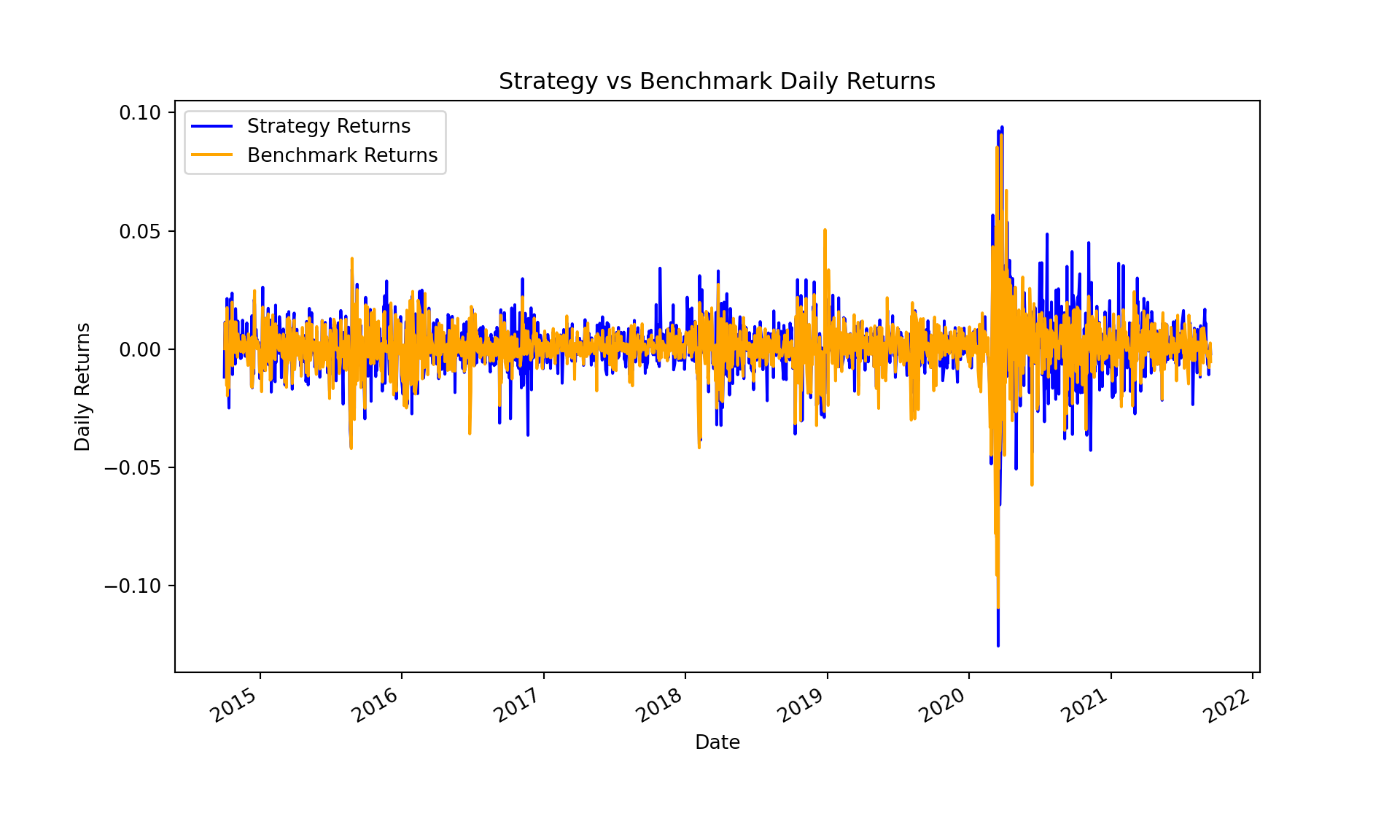
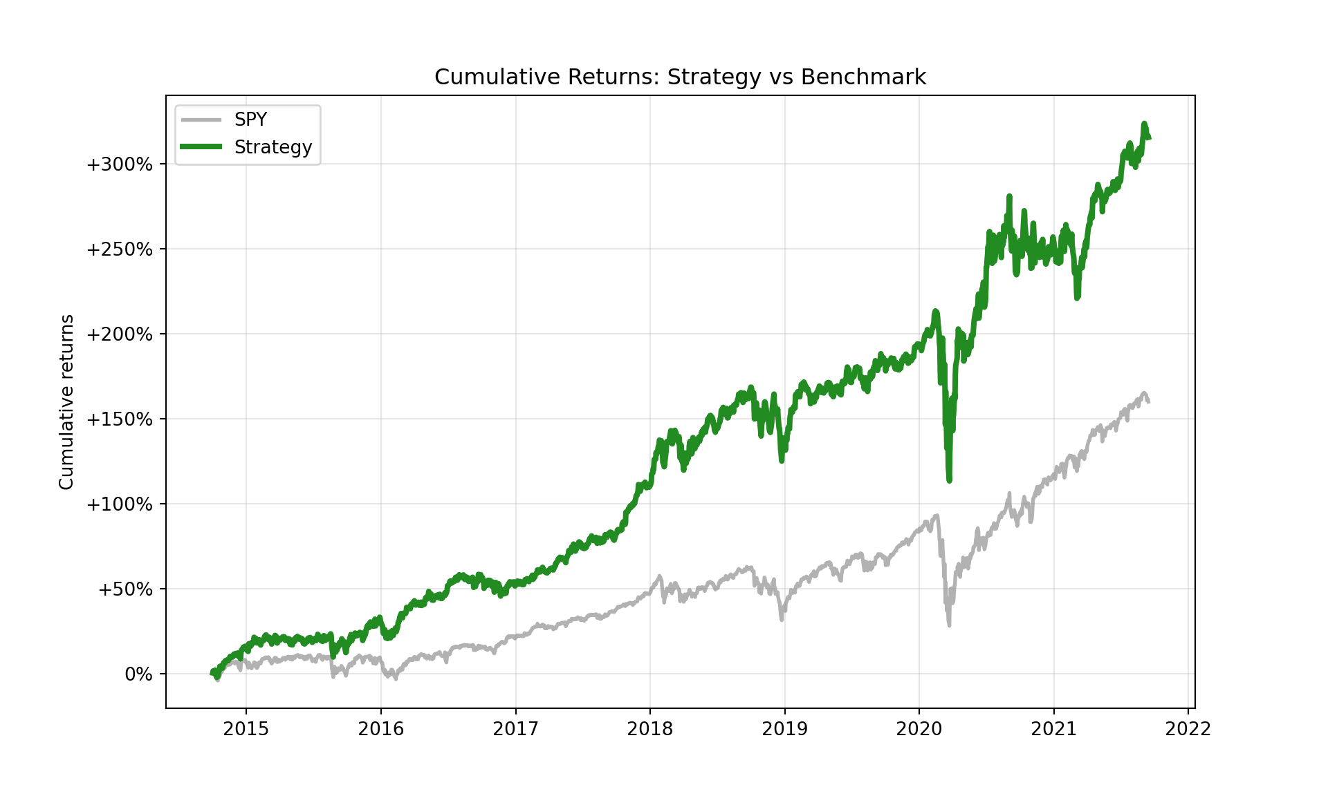
Backtest engine: Apply weights from the next open (to avoid look-ahead bias) and compare to SPY, which is an ETF that tracks the S&P 500 index.
Evaluation: Visualize the cumulative returns of the strategy vs the benchmark.

Note: this is one of the simplest possible backtests. One of the main limitations is that it evaluates the strategy on one path, whereas the real world is much more volatile and uncertain. For a survey on more advanced techniques, see this paper.

Generate Rolling Max-Sharpe Weights

We use the daily_returns function and symbols list created earlier to generate the rolling max-Sharpe weights. Some parameters:

TRADING_DAYS = 253
LOOKBACK_YEARS = 3 
REBAL_FREQ = pd.tseries.offsets.BusinessMonthEnd() 
BENCH_TICKER = "SPY"

Show code

TRADING_DAYS = 253 
LOOKBACK_YEARS = 3 
REBAL_FREQ = pd.tseries.offsets.BusinessMonthEnd()  
BENCH_TICKER = "SPY" 

def max_sharpe_weights(window_returns: pd.DataFrame) -> np.ndarray:
    """
    Long-only, sum-to-1 max-Sharpe optimization.

    Parameters
    ----------
    window_returns : pd.DataFrame
        DataFrame of returns for the assets in the window.

    Returns
    -------
    np.ndarray
        Weights for the assets that maximize the Sharpe ratio.
    """
    mu, cov = window_returns.mean() * TRADING_DAYS, window_returns.cov() * TRADING_DAYS
    n, x0 = len(mu), np.full(len(mu), 1 / len(mu))

    def neg_sr(w) -> float:
        ret = w @ mu.values
        vol = np.sqrt(w @ cov.values @ w) + 1e-12  # Tiny jitter to avoid division by zero
        return -ret / vol

    constraints = [{"type": "eq", "fun": lambda w: w.sum() - 1}]
    bounds = [(0, 1)] * n
    opt_results = sco.minimize(neg_sr, x0, method="SLSQP", bounds=bounds, constraints=constraints)
    # Default to equal weights if optimization fails
    return opt_results.x if opt_results.success else x0

We resample the daily returns to get the business month-end returns, which will be used for rebalancing. The lookback period is defined as LOOKBACK_YEARS * TRADING_DAYS, which gives us the number of trading days in the lookback period. We then compute the max-Sharpe weights for each month-end date using the max_sharpe_weights function defined above.

Show code

lookback_days = LOOKBACK_YEARS * TRADING_DAYS
month_ends = daily_returns.resample(REBAL_FREQ).last().index
month_ends

DatetimeIndex(['2011-09-30', '2011-10-31', '2011-11-30', '2011-12-30',
               '2012-01-31', '2012-02-29', '2012-03-30', '2012-04-30',
               '2012-05-31', '2012-06-29',
               ...
               '2020-12-31', '2021-01-29', '2021-02-26', '2021-03-31',
               '2021-04-30', '2021-05-31', '2021-06-30', '2021-07-30',
               '2021-08-31', '2021-09-30'],
              dtype='datetime64[ns]', name='Date', length=121, freq='BME')

Rolling through the month-end dates, we compute the max-Sharpe weights for each month-end date using the max_sharpe_weights function. The assumption is that the weights are re-optimized at each month-end based on the past LOOKBACK_YEARS of data.

The results are first stored in a dictionary where the keys are the rebalance dates and the values are the weights for each asset at that date:

Show code

weight_snapshots = {}
for d in month_ends:
    window = daily_returns.loc[:d].tail(int(lookback_days))
    if len(window) < lookback_days:  # Skip until we have full history
        continue
    weight_snapshots[d] = max_sharpe_weights(window)

weights_data = pd.DataFrame.from_dict(
    weight_snapshots, orient="index", columns=symbols
).sort_index()

weights_data.index.name = "rebalance_date"

	XOM	SHW	JPM	AEP	AMZN	BA	AMT	DD	TSN
2014-09-29 20:00:00	0.1150270	0.0895104	0.0000000	0.1313895	0.0000000	0.4041047	0.0000000	0.1427702	0.1171983
2014-10-30 20:00:00	0.2192979	0.0747711	0.0000000	0.0887031	0.0000000	0.3417924	0.0000000	0.1046540	0.1707815
2014-11-27 19:00:00	0.1820858	0.0962276	0.0000000	0.1019916	0.0018596	0.3204046	0.0000000	0.0853359	0.2120948
2014-12-30 19:00:00	0.2282962	0.0203970	0.0000000	0.0555508	0.0357932	0.3845636	0.0208262	0.0509807	0.2035923
2015-01-29 19:00:00	0.2732742	0.0000000	0.0126188	0.1136174	0.0000000	0.3386744	0.0000000	0.0626928	0.1991224
2015-02-26 19:00:00	0.1967416	0.0001810	0.0333682	0.1407724	0.0000000	0.3444375	0.0000000	0.0937190	0.1907803

In the dataframe above, each row corresponds to a month-end rebalance date, and each column corresponds to an asset in the portfolio. The values are the optimized weights (with respect to maximizing the Sharpe ratio) assigned to each asset at that rebalance date. By construction, all weights are $\geq 0$ and sum to 1, so no leverage is assumed.

We can verify that the weights sum to 1 for each rebalance date:

Show code

np.allclose(weights_data.to_numpy().sum(axis=1), 1)

True

Transform Weights into Daily Returns

Next, we need to transform the monthly weights into daily weights again. This is done by forward-filling the weights until the next rebalance date, and then shifting the weights by one day to ensure that the weights are applied from the next trading day after the signal is generated. This avoids look-ahead bias, as we do not use the weights from the same day they are calculated.

Without shift(1), we would be using information from day T to make decisions on day T. This creates an unrealistic scenario where we’re using the same day’s market close data to decide the portfolio weights for that same day. In reality:

The optimal weights are calculated using data available at the END of day T
We can only implement those weights starting from day T+1
There’s always a delay between signal generation and execution

Show code

daily_weights = (
    weights_data.reindex(daily_returns.index, method="ffill")  # Hold until next rebalance
    .shift(1)  # Start the day *after* the signal
    .dropna(how="all")
)

	XOM	SHW	AEP	BA	DD	TSN
2014-09-30 20:00:00	0.115027	0.0895104	0.1313895	0.4041047	0.1427702	0.1171983
2014-10-01 20:00:00	0.115027	0.0895104	0.1313895	0.4041047	0.1427702	0.1171983
2014-10-02 20:00:00	0.115027	0.0895104	0.1313895	0.4041047	0.1427702	0.1171983
2014-10-05 20:00:00	0.115027	0.0895104	0.1313895	0.4041047	0.1427702	0.1171983
2014-10-06 20:00:00	0.115027	0.0895104	0.1313895	0.4041047	0.1427702	0.1171983
2014-10-07 20:00:00	0.115027	0.0895104	0.1313895	0.4041047	0.1427702	0.1171983

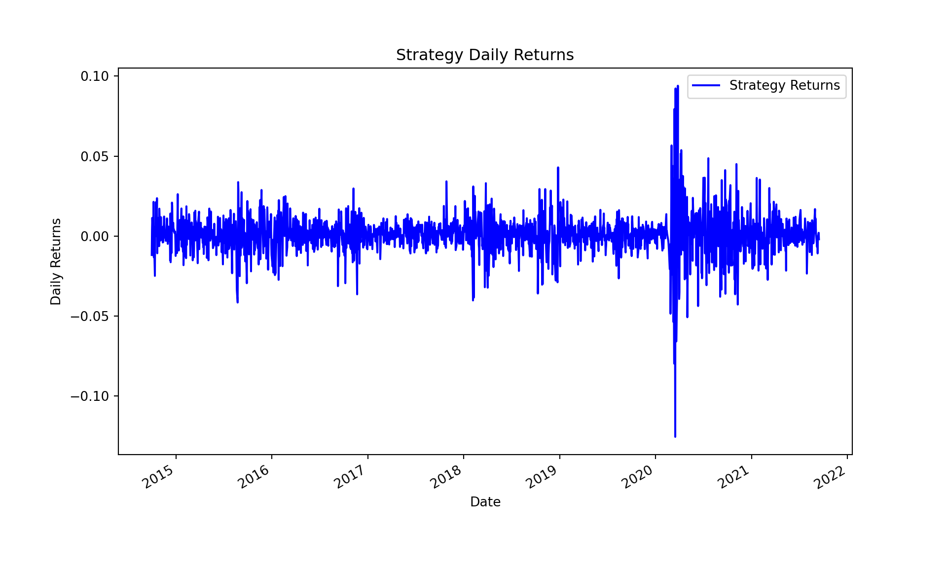
The daily returns of the strategy can be obtained by multiplying the daily weights with the daily returns of the assets. The result is a series of daily returns for the strategy, which we can then use to evaluate the performance of the portfolio.

Show code

strategy_returns = (daily_weights * daily_returns.loc[daily_weights.index]).sum(axis=1)
strategy_returns.name = "max_sharpe_monthly"

fig, ax = plt.subplots(figsize=(10, 6))
strategy_returns.plot(ax=ax, label="Strategy Returns", color="blue")
ax.set_title("Strategy Daily Returns")
ax.set_ylabel("Daily Returns")
ax.set_xlabel("Date")
ax.legend()
plt.show()

Benchmark Returns

Download the benchmark data and compute the daily returns:

Show code

bench_prices = yf.download(
    BENCH_TICKER, 
    start=str(strategy_returns.index.min().date()), 
    auto_adjust=False
)["Adj Close"]


[*********************100%***********************]  1 of 1 completed

Show code

benchmark_returns = bench_prices.pct_change().reindex(strategy_returns.index).dropna()
benchmark_returns = benchmark_returns.squeeze("columns")
benchmark_returns.name = BENCH_TICKER

fig, ax = plt.subplots(figsize=(10, 6))
strategy_returns.plot(ax=ax, label="Strategy Returns", color="blue")
benchmark_returns.plot(ax=ax, label="Benchmark Returns", color="orange")
ax.set_title("Strategy vs Benchmark Daily Returns")
ax.set_ylabel("Daily Returns")
ax.set_xlabel("Date")
ax.legend()
plt.show()

Plotting Cumulative Returns

First, align the indices of both series to ensure they cover the same dates and convert the indices to tz-aware datetime objects.

Show code

strategy_returns, benchmark_returns = strategy_returns.align(
    benchmark_returns, join="inner"  # Keep only dates common to both
)

strategy_returns.index  = strategy_returns.index.tz_localize("UTC")
benchmark_returns.index = benchmark_returns.index.tz_localize("UTC")

At this point we have two aligned pd.Series objects:

object	description
`strategy_returns`	daily returns of the rolling Markowitz strategy
`benchmark_returns`	daily returns of SPY

We can now plot the cumulative returns of the strategy and the benchmark, with a clear distinction between the in-sample and out-of-sample periods. The cumulative returns are calculated by taking the cumulative product of the daily returns plus one.

Show code

def plot_rolling_returns(
    returns: pd.Series,
    benchmark: pd.Series | None = None,
    live_start_date: str | pd.Timestamp | None = None,
    logy: bool = False,
    ax: plt.Axes | None = None,
) -> plt.Axes:
    """
    Plot cumulative returns of a strategy with optional benchmark overlay.

    Parameters
    ----------
    returns : pd.Series
        Daily strategy returns (non-cumulative, index = DatetimeIndex).
    benchmark : pd.Series, optional
        Daily benchmark returns to overlay (same index as `returns`).
    live_start_date : str | pd.Timestamp, optional
        Date that separates backtest vs. live trading.
    logy : bool, default False
        Plot y-axis on log scale.
    ax : matplotlib.axes.Axes, optional
        Pre-existing axes to plot on.

    Returns
    -------
    ax : matplotlib.axes.Axes
        The axis containing the plot.
    """
    if ax is None:
        fig, ax = plt.subplots(figsize=(10, 6))

    cum_returns = (1 + returns).cumprod()

    if benchmark is not None:
        bench_cum = (1 + benchmark.reindex(cum_returns.index)).cumprod()
        ax.plot(
            bench_cum,
            lw=2,
            color="grey",
            alpha=0.6,
            label=benchmark.name if benchmark.name else "Benchmark",
        )

    if live_start_date is not None:
        live_start_date = pd.to_datetime(live_start_date).tz_localize(cum_returns.index.tz)
        is_mask = cum_returns.index < live_start_date
        oos_mask = cum_returns.index >= live_start_date

        ax.plot(cum_returns[is_mask], lw=3, color="forestgreen", label="Backtest")
        ax.plot(cum_returns[oos_mask], lw=3, color="red", label="Live")
    else:
        ax.plot(cum_returns, lw=3, color="forestgreen", label="Strategy")

    ax.set_yscale("log" if logy else "linear")

    # Custom percentage formatter
    def percentage_formatter(x, pos):
        if x == 1.0:
            return "0%"
        elif x < 1.0:
            return f"-{(1-x)*100:.0f}%" if (1-x)*100 >= 1 else f"-{(1-x)*100:.1f}%"
        else:
            return f"+{(x-1)*100:.0f}%" if (x-1)*100 >= 1 else f"+{(x-1)*100:.1f}%"
    
    ax.yaxis.set_major_formatter(ticker.FuncFormatter(percentage_formatter))
    
    # Force matplotlib to show more ticks by setting the locator
    if not logy:
        ax.yaxis.set_major_locator(ticker.MaxNLocator(nbins=8))
    
    ax.set_ylabel("Cumulative returns")
    ax.set_xlabel("")
    ax.legend(frameon=True)
    ax.grid(alpha=0.3)

    return ax

Show code

fig, ax = plt.subplots(figsize=(10, 6))
plot_rolling_returns(
    returns=strategy_returns,
    benchmark=benchmark_returns,
    live_start_date=None,
    logy=False,
    ax=ax,
)
ax.set_title("Cumulative Returns: Strategy vs Benchmark")
plt.show()

The visualization above shows the cumulative returns of the rolling max-Sharpe strategy compared to the benchmark. However, there are several practical gaps and limitations to consider:

Universe bias – We selected 12 tickers that survive the whole 10-year span. That removes delisted firms and understates real-world failure risk.
Transaction costs & slippage – Even at monthly turnover they can materially reduce the Sharpe ratio. The back-test currently assumes zero costs, which is not realistic.
Parameter robustness – We fix one look-back length (36 months). A robustness grid (e.g., 24–60 m) or a nested cross-validation loop would reveal sensitivity.