Recently, I came across a concept called function factory in Advance R, which allows one to create functions that return other functions as outputs. Why? I guess it is partly because R is at its heart a functional programming language. And, the function factory actually has many useful applications, particularly when it is used in tandem with the tidyverse’s graphics library ggplot2 and when it is used to implement statistical theories.

In this post, I want to document some of what I have learned in reading about the function factory and its cool applications. To accomplish that, a bit of theory on the R environments is required. The content of this post can be found in chapter 10 of Advance R. The function factory is kind of a quirky concept that I believe is part of what makes R unique, and so I recommend reading more about it in Hadley’s book. With that being said, let us get started.

The following packages are required for this post:

Hide Code

library(rlang)
library(knitr)
library(tidyverse)

What makes a function factory special?

The underlying key idea behind function factories can be succinctly expressed as follows:

The enclosing environment of the manufactured function is an execution environment of the function factory — Hadley Wickham

We can understand this better using an example. Suppose we have a function factory called power, which returns manufactured functions that raise their input arguments to different powers, contingent on the exp argument supplied to the factory function:

Hide Code

power <- function(exp) {
  # Force the evaluation of "exp"
  base::force(exp)

  # This is the last evaluated expression and so the function returns another function
  # It takes an input "x" and raises it to the power of "exp"
  # The argument "exp" is supplied as an argument to "power"
  function(x) {
    x^exp
  }
}

By varying on our inputs to exp via power, we can create a class of functions that behave differently:

Hide Code

square <- power(exp = 2)
cube <- power(exp = 3)

Let us see it in action:

Hide Code

square(x = 32)

[1] 1024

Hide Code

cube(x = 9)

[1] 729

As can be seen, these functions are exactly how we would expect them to behave. But why do they behave differently? From the looks of it, their function bodies are exactly the same:

Hide Code

square

function (x) 
{
    x^exp
}
<environment: 0x10f58a270>

Hide Code

cube

function (x) 
{
    x^exp
}
<bytecode: 0x10f00ed68>
<environment: 0x10f4900e0>

It turns out that the most important difference between these functions is that they have different enclosing or function environments (see the different environment addresses in the output above). The enclosing environments control how these functions scope for values of exp. Each time a function is executed in R, a new execution environment is created to host its execution. The first time we executed power to create square, an environment is created. Then, another execution environment of power is created when we generated cube. These two execution environments are the enclosing environments of square and cube. The rlang package contains functions that provide more insights into these relationships:

Hide Code

# Examine the environments associated with the function square
env_print(env = square)

<environment: 0x10f58a270>
Parent: <environment: global>
Bindings:
• exp: <dbl>

Hide Code

# Examine the environments associated with the function cube
env_print(env = cube)

<environment: 0x10f4900e0>
Parent: <environment: global>
Bindings:
• exp: <dbl>

As can be seen, there are two different environment addresses associated with these two functions, each of which was an execution environment of power. These environments have the same parent— the enclosing or function environment of power, which is also the global environment in which power was created. Both the environments for square and cube contain a binding to exp; we can access the value of exp to see ultimately why these two functions behave differently:

Hide Code

# Examine the value of "exp" in the enclosing environment of square
fn_env(fn = square)[["exp"]]

[1] 2

Hide Code

# Examine the value of "exp" in the enclosing environment of cube
fn_env(fn = cube)[["exp"]]

[1] 3

So, in short, square and cube behave differently since the names exp in their enclosing environments are bound to different values.

Diagrams

These relationships between a function factory and its manufactured functions can be analyzed diagrammatically. The components of the diagram below are:

The boat-like structures are the functions, i.e. power, square, and cube.
The global environment is represented by the rectangular shape labeled “R_GlobalEnv.”
The execution environments of power or, equivalently, the enclosing environments of square and cube are symbolized by the grey boxes each of which has a binding from the name exp to a double vector object.
The black arrows indicate bindings either from names to objects— be it a function object like power or a vector object like 2— or from a function object to its enclosing environment— be it when power binds its enclosing global environment or when square and cube bind their respective enclosing environments.
The blue arrows indicate relationships between environments and their parent environments. The blue arrow always goes in a one-way direction from the child environment to the parent environment.

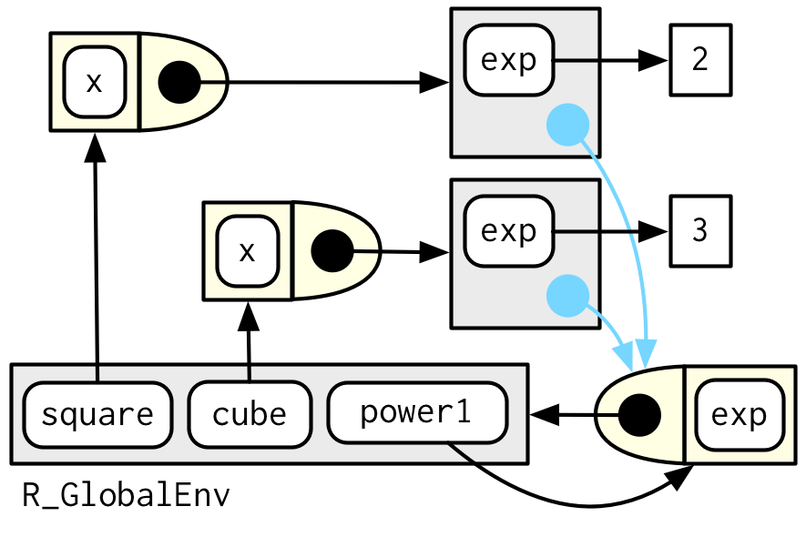
From the diagram, the relationships can be summarized as follows:

The function power (bottom-right) binds the global environment, which is where it was created. The global environment has a binding from the name “power1” to the function object (boat-like structure). These two bindings are made clear in the diagram by the black arrows pointing from power to global and from global to power.
The global environment has in its bag two other bindings from the names “square” and “cube” to the function objects located in the top left of the diagram.
The parent of the execution environments of power is the function or enclosing environment of power. The blue arrows going from the grey boxes to the bloat-like structure representing power reveal these relationships.
- The two execution environments are bound by the function objects square and cube, which is why there are black arrows pointing from their structures to the grey boxes in the diagram above.
- The two execution environments each has its own binding from the name exp to the double vector objects; this is indicated by the black arrows pointing from the grey boxes to the values 2 and 3.

Execution environment of a manufactured function

What happens when we execute square and cube? The answer is— same as before. Each time a function is called, an environment is created to host its execution. The parent of this execution environment is the enclosing or function environment of the function, which is determined by where it is created. Therefore, calling square and cube individually generates execution environments of their own. And the parents of these execution environments are the enclosing or function environments of square and cube, respectively. For instance, let us look at square. We can explicitly return the execution environment of square by using the current_env() function from the rlang package:

Hide Code

# New power function factory
power <- function(exp) {
  # Force the evaluation of "exp"
  force(exp)

  function(x) {
    x^exp
    # We explicitly force the return of the execution environment of any manufactured function
    current_env()
  }
}
# New square function
square <- power(exp = 2)

Now, whenever we execute square, it will return the execution environment of square:

Hide Code

# Raise 10 to the power of 2
square(x = 10) %>%
  # Execution and its parent environment
  env_print()

<environment: 0x11a54eb00>
Parent: <environment: 0x11a25f798>
Bindings:
• x: <dbl>

In the output above, the first line represents the address of the execution environment of square. The last line shows that there is a binding from the name “x” to a double vector object (“dbl” is short for double), which is the argument that we supplied to the function square, $x = 10$ . The second line of the output above is of the utmost importance and it should make sense— it is the enclosing environment of square. How can we be sure? Well, we can manually check the enclosing environment of square:

Hide Code

env_print(env = square)

<environment: 0x11a25f798>
Parent: <environment: global>
Bindings:
• exp: <dbl>

As can be seen, the first line of the output above indeed matches with the second line of the output from earlier. We now have a proof of the relationship between the execution environment and the enclosing environment of a manufactured function. And, it is no different than the relationships between environments of any other functions.

Diagram

But can we expound on the execution environment of a manufactured function more? Perhaps we can see the relationships more clearly via a diagram:

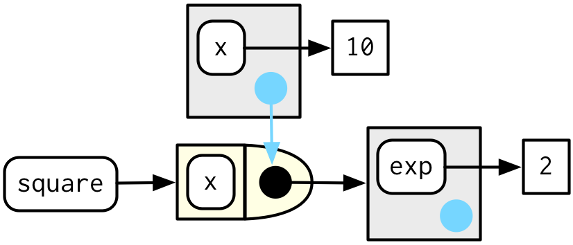
The relationships in the diagram can be summarized as follows:

The boat-like structure represents square (clearly, the name square is bound to this function object via the black arrow). The function also binds its enclosing environment, which is the grey box containing a binding exp. Recall that this environment was also one of the execution environments of power. However, in this diagram, we are zooming in to get a more focused view on the manufactured function square.
What we have proved in the section above is precisely the relationship between the grey box on top of square and the grey box to the right of square. The grey box on top is indeed the execution environment of square (with the blue arrow pointing to the function object), and the grey box to the right is its enclosing environment. When square is executed, it scopes for the value of “x” in the execution environment, $x = 10$ , and the value of exp in its enclosing environment, which is 2.

And, this is what makes a function factory special. The behavior of any manufactured function is powered by the execution environment of the factory function, which is different each time the factory function is used to create a manufactured function. With this core idea under our belt, we will be able to produce some elegant solutions when it comes to creating formatter functions for graphs or statistical functions used to transform, sample, or estimate data. We will tackle all of these in the next few posts.