Implementing Mathematical Concepts in R

In my first post, we will be implementing some interesting mathematical concepts in R.

library(tidyverse)
library(memoise)
library(rlang)
library(knitr)
library(purrr)

The Binomial Theorem

$$\begin{array}{r}(x+y{)}^n=\sum _{k=0}^n(\genfrac{}{}{0ex}{}{n}{k})x^k{y}^{n-k}\end{array}$$

Expanding:

$$\begin{array}{r}(x+y{)}^n=(\genfrac{}{}{0ex}{}{n}{0})x^0{y}^{n-0}+(\genfrac{}{}{0ex}{}{n}{1})x^1{y}^{n-1}+(\genfrac{}{}{0ex}{}{n}{2})x^2{y}^{n-2}+...\\ +(\genfrac{}{}{0ex}{}{n}{n-1})x^{n-1}{y}^{n-(n-1)}+(\genfrac{}{}{0ex}{}{n}{n})x^n{y}^{n-n}\end{array}$$

In R, we can tackle the implementation of the Binomial Theorem in three parts:

• The binomial coefficient
• raising the real number $x$ to the vector of powers $k$
• Raising the real number $y$ to the vector of powers $n-k$

binomial_theorem <- function(x, y, n) {
  # Create a sequence from k = 0 to k = n
  seq_k_n <- seq.int(from = 0, to = n, by = 1)


  # Pre-allocate container for storing coefficients
  binom_coeffs <- vector(mode = "double", length = n + 1)
  # Binomial coefficients
  binom_coeffs <- map_dbl(.x = seq_k_n, .f = choose, n = n)


  # Pre-allocate container for storing the x's
  vector_of_x <- vector(mode = "double", length = n + 1)
  # Raise x to the power of y
  vector_of_x <- x^(seq_k_n)


  # Pre-allocate container for storing the y's
  vector_of_y <- vector(mode = "double", length = n + 1)
  # Raise y to the power of n-k
  vector_of_y <- y^(n - (seq_k_n))


  # Product of the two vectors and their coefficients
  prod <- binom_coeffs * vector_of_x * vector_of_y

  # Summation operator
  result <- sum(prod)
  result
}

---

Let’s see it in action:

# Test
x <- 924
y <- 23
n <- 39
# Compute by hand
(x + y)^n

[1] 1.195774e+116

# Compute using custom function
binomial_theorem(x = x, y = y, n = n)

[1] 1.195774e+116

As can be seen, the results are exactly the same.

---

Pascal’s Triangle

Directly related to the Binomial coefficient is Pascal’s triangle, whose entries in each row are usually staggered relative to the numbers in the adjacent rows.

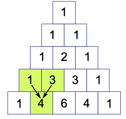
To implement Pascal’s triangle, we will use a for loop. Our goal is to write a program that finds the next row of Pascal’s triangle, given the previous rows.

# Finding the (n + 1)th row of a Pascal's triangle given n rows that precede it
pascal_triangle_n_plus_1 <- function(x) {
  if (!is.list(x)) {
    rlang::abort(message = "The input object must a be a list containing the rows of Pascal's Triangle.")
  }

  # Set n equal to depth of the input list "x", that is, the number of elements in x, where each represents a row
  n <- length(x)
  # Extract the last element (the nth row) from the input list "x" and store it as a new variable x_n
  # Use [[ to extract the value rather than a sub-list
  x_n <- x[[n]]
  # Repeat the integer "1" (n + 1) times
  # Note that the (n + 1)th  row has (n + 1) elements beginning and ending with 1
  x_n_plus_1 <- rep(x = 1, times = n + 1)

  # Loop to add all adjacent pairs in the nth row to obtain the (n + 1)th row
  # Start with the second element and end with second to last element of each row
  # This is because the first and last numbers in any given row are always 1
  if (n > 1) {
    # This is the prefix form of for loop
    `for`(
      var = i,
      seq = 2:n,
      action = x_n_plus_1[[i]] <- x_n[[i - 1]] + x_n[[i]]
    )
  }

  # Append the (n + 1)th row to the list object
  base::append(x, values = list(x_n_plus_1))
}

---

Let’s see it in action:

# Create a Pascal's Triangle with 4 rows
x <- list(c(1), c(1, 1), c(1, 2, 1), c(1, 3, 3, 1))
# Row 5
x <- pascal_triangle_n_plus_1(x = x)
x[[5]]

[1] 1 4 6 4 1

# Row 6
x <- pascal_triangle_n_plus_1(x = x)
x[[6]]

[1]  1  5 10 10  5  1

# We know that these row entries can be computed are the binomial coefficients 5 choose 0 thru 5 choose 5
map2_dbl(
  .x = rep(x = 5, times = 6),
  .y = seq.int(from = 0, to = 5, by = 1),
  .f = choose
)

[1]  1  5 10 10  5  1

---

Fibonacci with Memoization

The Fibonacci sequence is defined recursively, where the first two values are given by convention, $f(0)=0$, $f(1)=1$, and the rest are calculated as follows:

$$\begin{array}{r}f(n)=f(n-1)+f(n-2)\end{array}$$

However, a naive recursive implementation is inefficient because it repeatedly recalculates the same values during each step. Using memoise, we can cache previous computations, significantly speeding up the process.

fib <- function(n) {
  if (n < 2) {
    return(1)
  }
  fib(n - 2) + fib(n - 1)
}

# Testing the naive implementation
system.time(fib(31))

   user  system elapsed 
  0.617   0.003   0.619 

Memoizing the function allows us to compute Fibonacci numbers more efficiently.

fib_memo <- memoise::memoise(function(n) {
  if (n < 2) {
    return(1)
  }
  fib_memo(n - 2) + fib_memo(n - 1)
})

# Testing the memoized implementation
system.time(fib_memo(31))

   user  system elapsed 
  0.009   0.000   0.009 

By caching the results, we avoid redundant calculations, improving performance for large inputs. Furthermore, calling the memoized function for the same input or the next input will be much faster than the naive implementation.

system.time(fib_memo(32))

   user  system elapsed 
  0.001   0.000   0.000 

system.time(fib(32))

   user  system elapsed 
  0.868   0.004   0.872 

---

Newton-Raphson Method

The Newton-Raphson method is an iterative numerical method for finding the roots (or zeros) of a real-valued function. The method uses the idea of linear approximation: at each iteration, the method refines the guess for the root by using the slope (derivative) of the function.

Given a function $f(x)$ and its derivative $f^{\prime }(x)$, the Newton-Raphson iteration formula is:

$$\begin{array}{r}{x}_{n+1}=x_n-\frac{f(x_n)}{f^{\prime }(x_n)}\end{array}$$

This formula is applied repeatedly, starting from an initial guess $x_0$, until the difference between successive approximations is less than a predefined tolerance $\epsilon$, i.e.,

$$\begin{array}{r}|x_{n+1}-x_n|<\epsilon \end{array}$$

---

The implementation below has some slight overhead due to our storing the intermediate steps in a vector, but this is a small price to pay for the added functionality.

newton_raphson <- function(f, f_prime, x0, tol = 1e-8, max_iter = 100) {
  # Define a function that applies a single Newton-Raphson step
  x <- x0
  steps <- numeric(max_iter + 1) # Preallocate space to store the steps
  steps[[1]] <- x0

  for (i in seq_len(max_iter)) {
    # Perform a Newton-Raphson step
    x_new <- x - f(x) / f_prime(x)
    steps[[i + 1]] <- x_new
    # If the tolerance condition is met, stop the iteration
    if (abs(x_new - x) < tol) {
      steps <- steps[1:(i + 1)] # Truncate the steps to only valid iterations
      break
    }
    x <- x_new
  }
  return(steps)
}

As an example, let’s find the root of the function:

$$\begin{array}{r}f(x)=x^3-2x-5\end{array}$$

and

$$\begin{array}{r}{f}^{\prime }(x)=3x^2-2\end{array}$$

f <- function(x) x^3 - 2 * x - 5
f_prime <- function(x) 3 * x^2 - 2
x_vals <- seq(-10, 10, by = 0.1)
y_vals <- map_dbl(x_vals, ~ f(.x))

ggplot(data.frame(x = x_vals, y = y_vals), aes(x = x, y = y)) +
  geom_line() +
  geom_hline(yintercept = 0, linetype = "dashed") +
  labs(
    title = "Graph of f(x) = x^3 - 2x - 5",
    x = "x",
    y = "f(x)"
  ) +
  theme_minimal()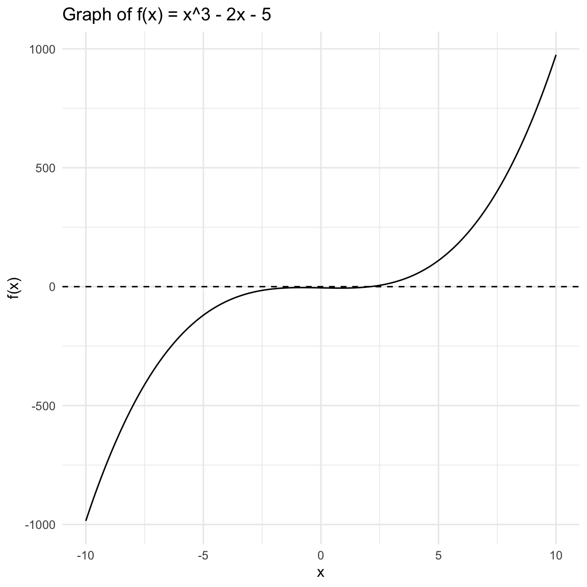

We will use an initial guess of $x_0=20$ and a tolerance of $\epsilon =1e-8$:

intermediate_steps <- newton_raphson(f = f, f_prime = f_prime, tol = 1e-8, x0 = 20, max_iter = 100)

The chart below shows the convergence of the Newton-Raphson method to the root of the function $f(x)$:

data <- data.frame(
  iteration = 1:length(intermediate_steps),
  approximations = intermediate_steps
)

ggplot(data, aes(x = iteration, y = approximations)) +
  geom_line() +
  geom_point() +
  labs(
    title = "Convergence of Newton-Raphson Method",
    x = "Iteration",
    y = "Approximation of Root"
  ) +
  theme_minimal()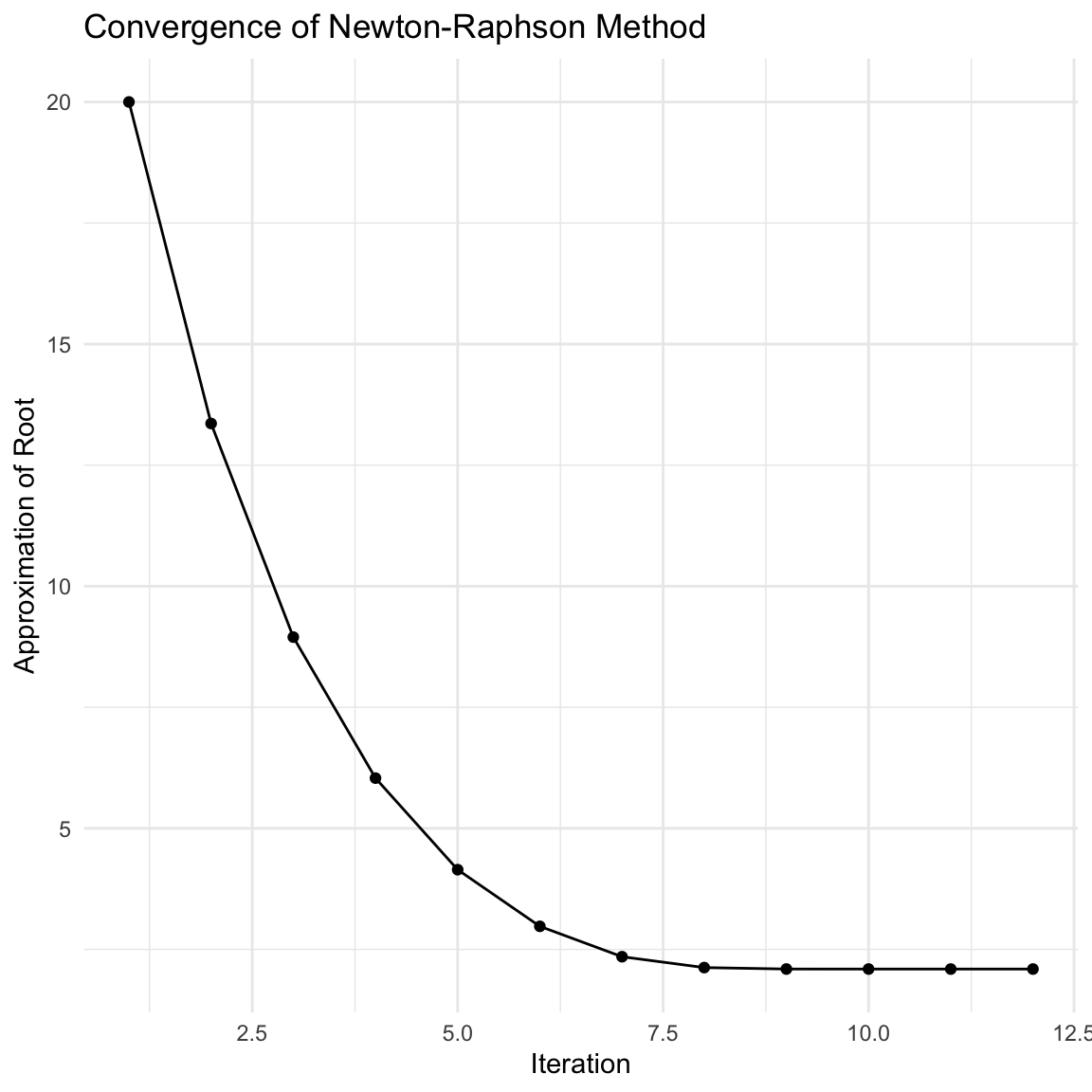

That’s it for my first post!